For real world vision or Robotic operations it is sometimes necessary to transform between coordinates in different coordinate systems. In this tutorial we will transform a 3D spiral from one coordinate system to another. The coordinate systems are specified in terms of their position in Cartesian space and converted to a vectorial representation.
First let us create and display the spiral
t = 0:pi/50:10*pi;
st = sin(t);
ct = cos(t);
The spiral is in 3D but we need a 4D matrix to perform the matrix transformations, so we also add a row of ones to it
spiral = [st; ct; t; ones(501,1)']
Ok, lets plot the relevant data
plot3(spiral(1,:), spiral(2,:), spiral(3,:), 'b')
we use the hold on command to keep plotting to the same chart
hold on
We are going to translate this spiral from its world coordinates to another local coordinate system
the coordinates are specified by a matrix = [X1, X2, X3, Y1, Y2, Y3, Z1, Z2, Z3]
world = [1,0,0;0,1,0;0,0,1]
local = [3,6,3;3,3,6;3,3,0]
The 3,3,0 in the last row (Z axis) of the matrix creates a 45 degree plane
Lets turn our local coordinate system into a vector
local_vector = zeros(3,3)
local_vector(:,1) = local(:,2)-local(:,1)
local_vector(:,2) = local(:,3)-local(:,1)
local_vector(:,3) = cross(local_vector(:,1),local_vector(:,2))
The vectors should be normalised to unit length like our world vector is
local_vector(:,1) = local_vector(:,1)/norm(local_vector(:,1))
local_vector(:,2) = local_vector(:,2)/norm(local_vector(:,2))
local_vector(:,3) = local_vector(:,3)/norm(local_vector(:,3))
Now we have to create our transform matrix using the dot product between our world and local vectors, this sets up the skew, reflection, rotation elements
transform = zeros(4,4)
transform(1,1) = dot(world(1,:), local_vector(1,:))
transform(1,2) = dot(world(1,:), local_vector(2,:))
transform(1,3) = dot(world(1,:), local_vector(3,:))
transform(2,1) = dot(world(2,:), local_vector(1,:))
transform(2,2) = dot(world(2,:), local_vector(2,:))
transform(2,3) = dot(world(2,:), local_vector(3,:))
transform(3,1) = dot(world(3,:), local_vector(1,:))
transform(3,2) = dot(world(3,:), local_vector(2,:))
transform(3,3) = dot(world(3,:), local_vector(3,:))
we also add the translated origin of our coordinate system to the last column of the matrix, this performs the X,Y,Z translation
transform(1,4) = local(1,1)
transform(2,4) = local(2,1)
transform(3,4) = local(3,1)
transform(4,4) = 1
So using our transform we can rotate the spiral by 45 degrees and translate it by 3 in X and 3 in Y
tspiral = transform*spiral;
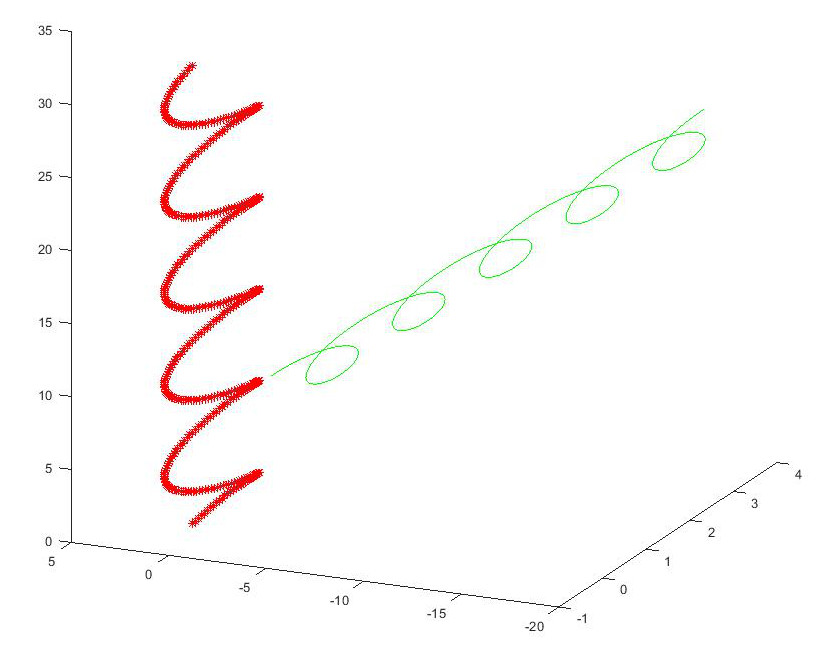
let’s plot it in green next to the original spiral
plot3(tspiral(1,:), tspiral(2,:), tspiral(3,:), 'g')
(you might want to rotate the plot axis now to see the two spirals in 3D)
now to get it back again we use the inverse of our transformation matrix
tunspiralInv = inv(transform)*tspiral;
and plot it using markers so we can see the orginal spiral beneath
plot3(tunspiralInv(1,:), tunspiralInv(2,:), tunspiralInv(3,:), ‘r*’)
The plot should look like this

For the mathematical details behind the transform, these MIT lecture notes provide an excellent explanation.
If you find the article useful, please feel free to post a link to it