Visualisation of irrational numbers as vectors

Beauty in irrationality?

Plotting irrational numbers (pi, e, sqrt2, golden ratio) as vectors allows their complexity to be visualised

I have always wanted to visualise irrational numbers. Our brains are capable of recognising patterns in nature and I wanted to know if these patterns could be visualised in irrational numbers, and whether beautiful patterns could be seen that could lead to an further understanding of the irrational nature of the numbers. Just found out after publishing this article that the idea has been round for a while! (here is an interesting blog article). Here I have extended the technique to 3 dimensions for better visualisation and give results and computer code.

Experimental Technique

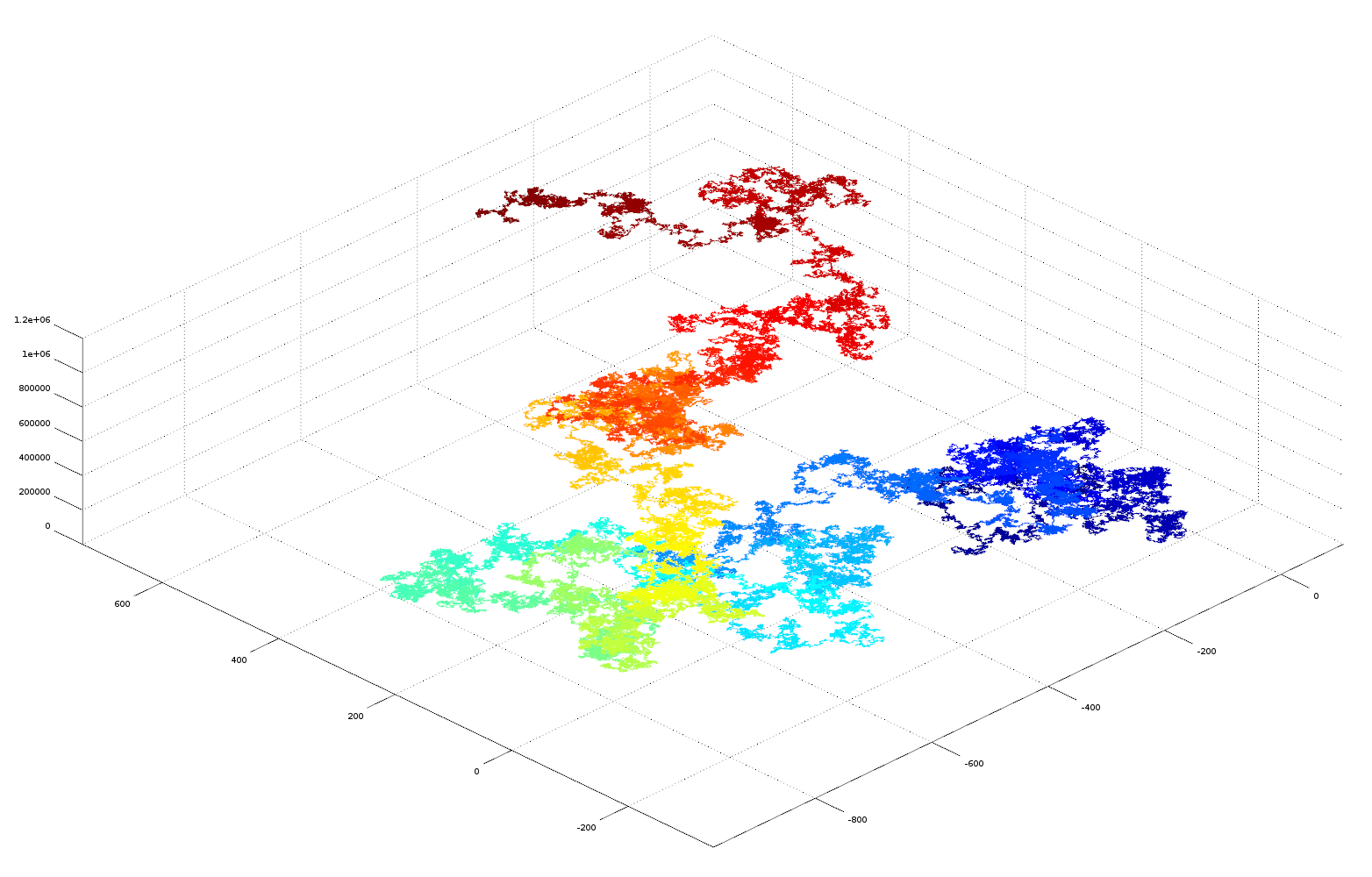
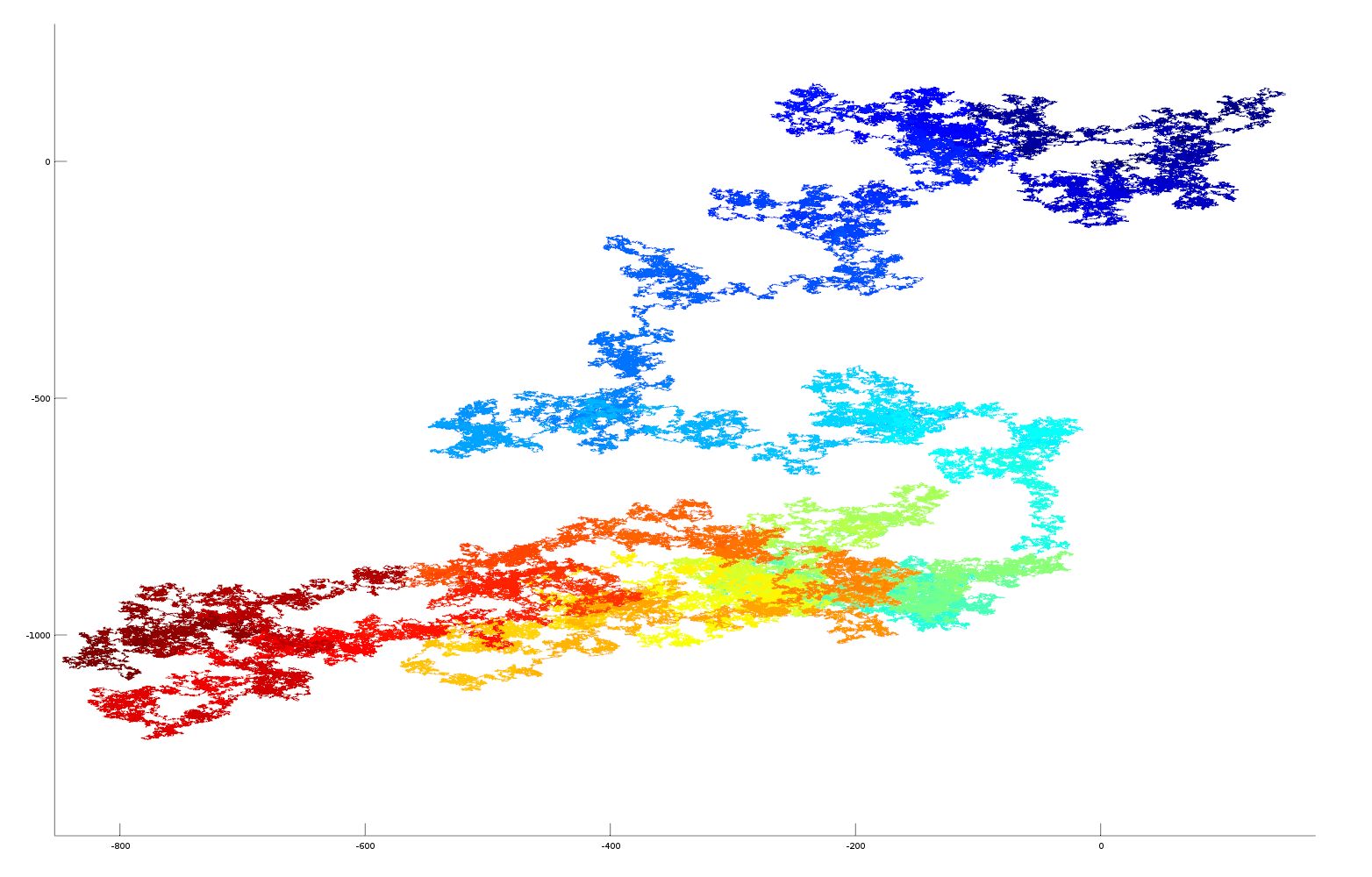
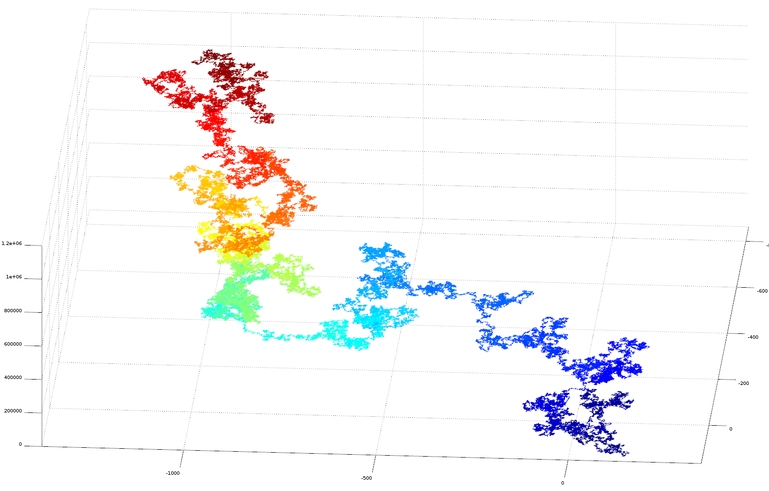
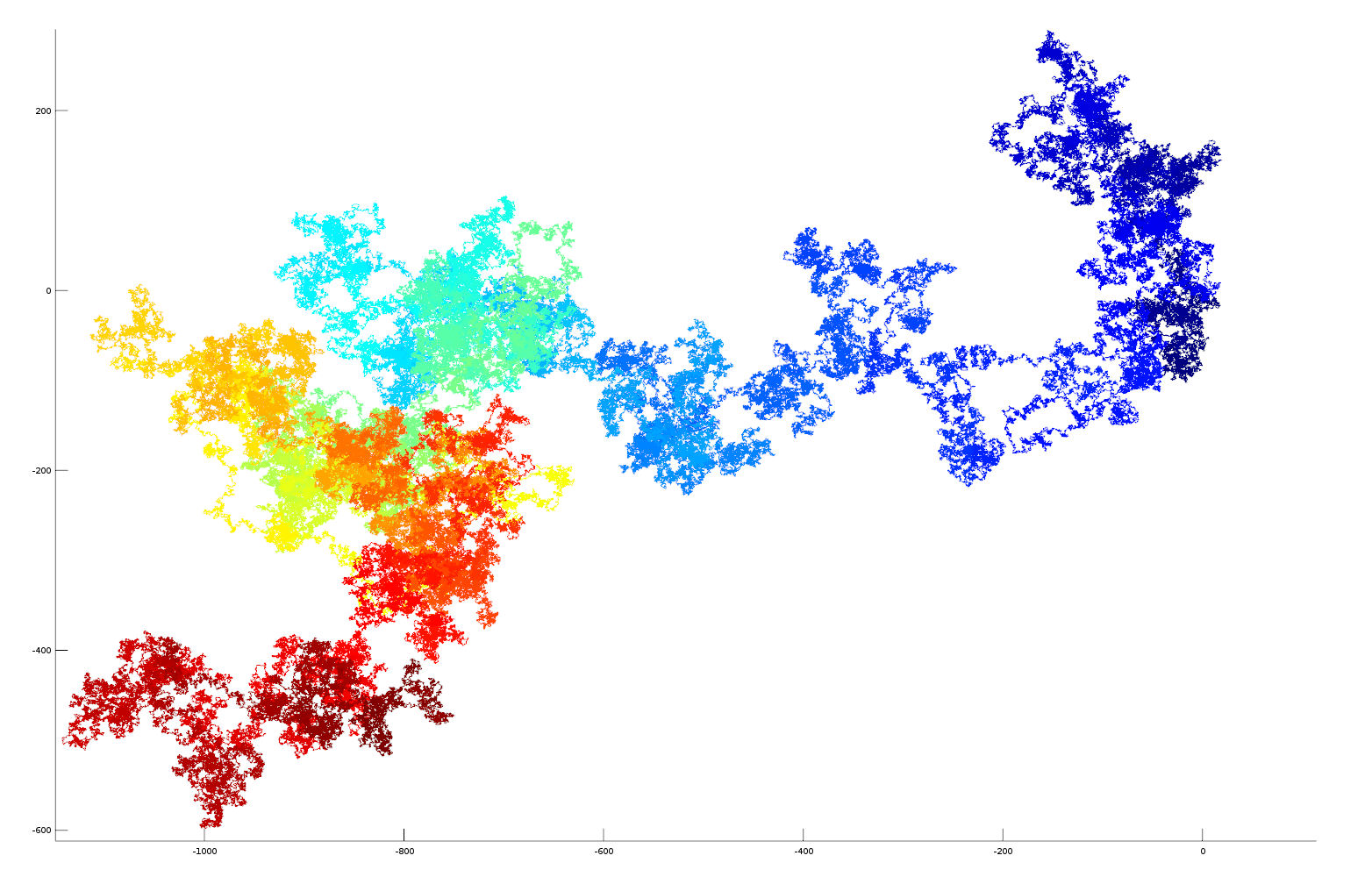
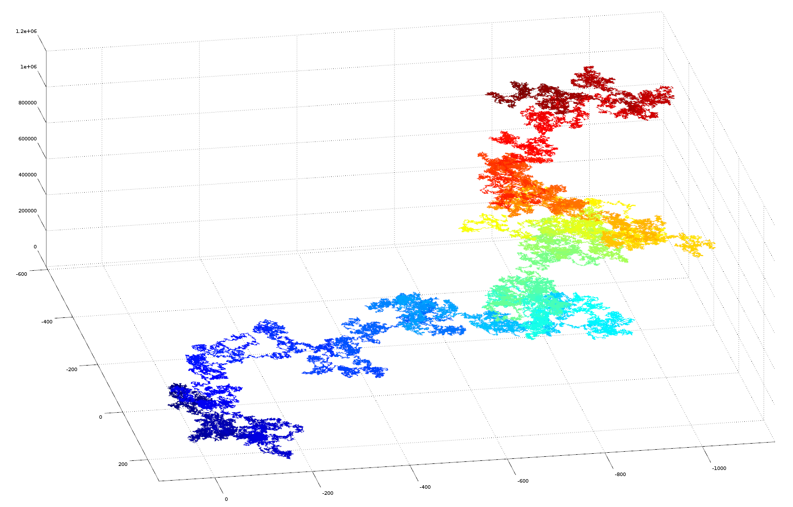
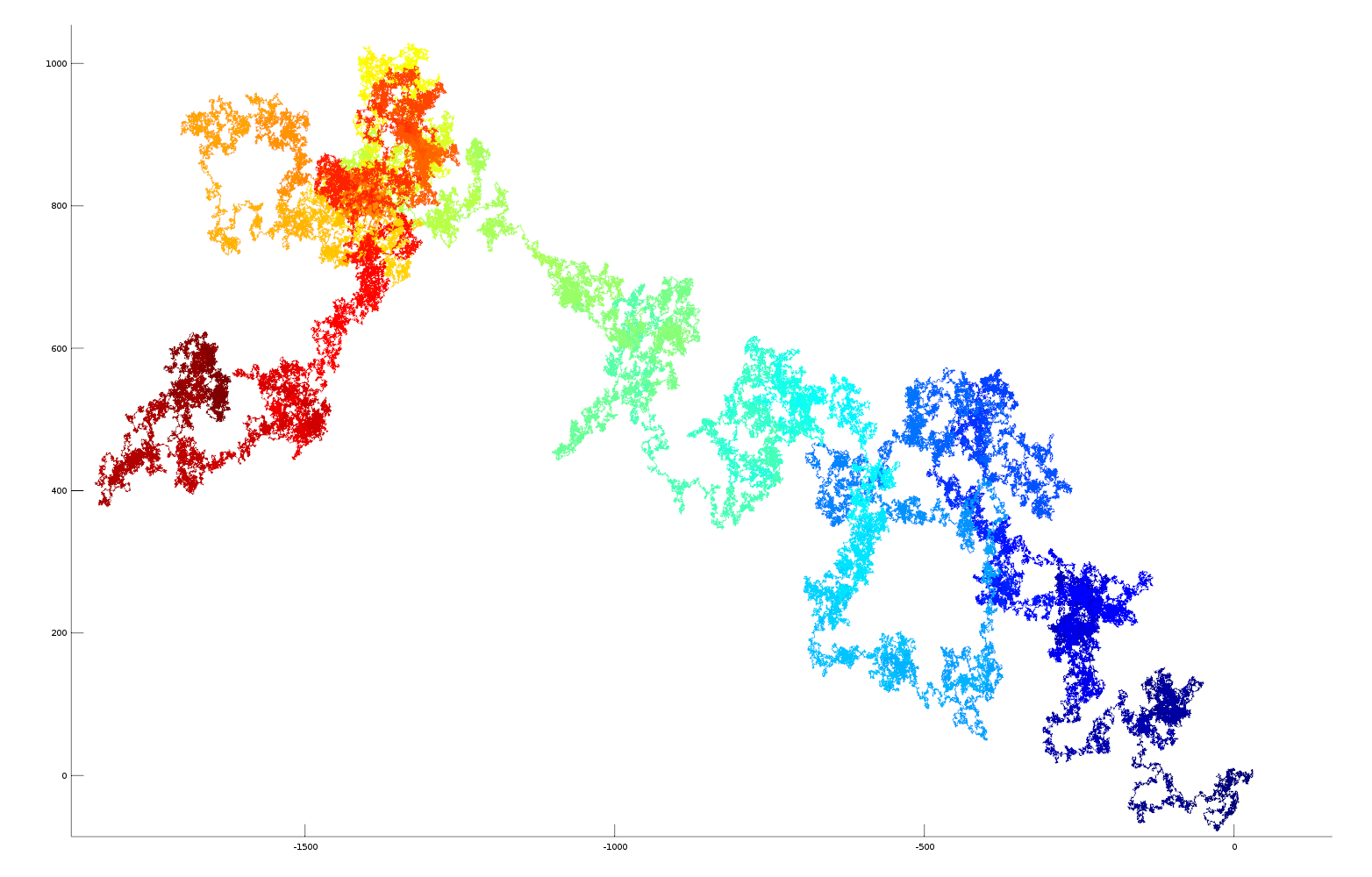
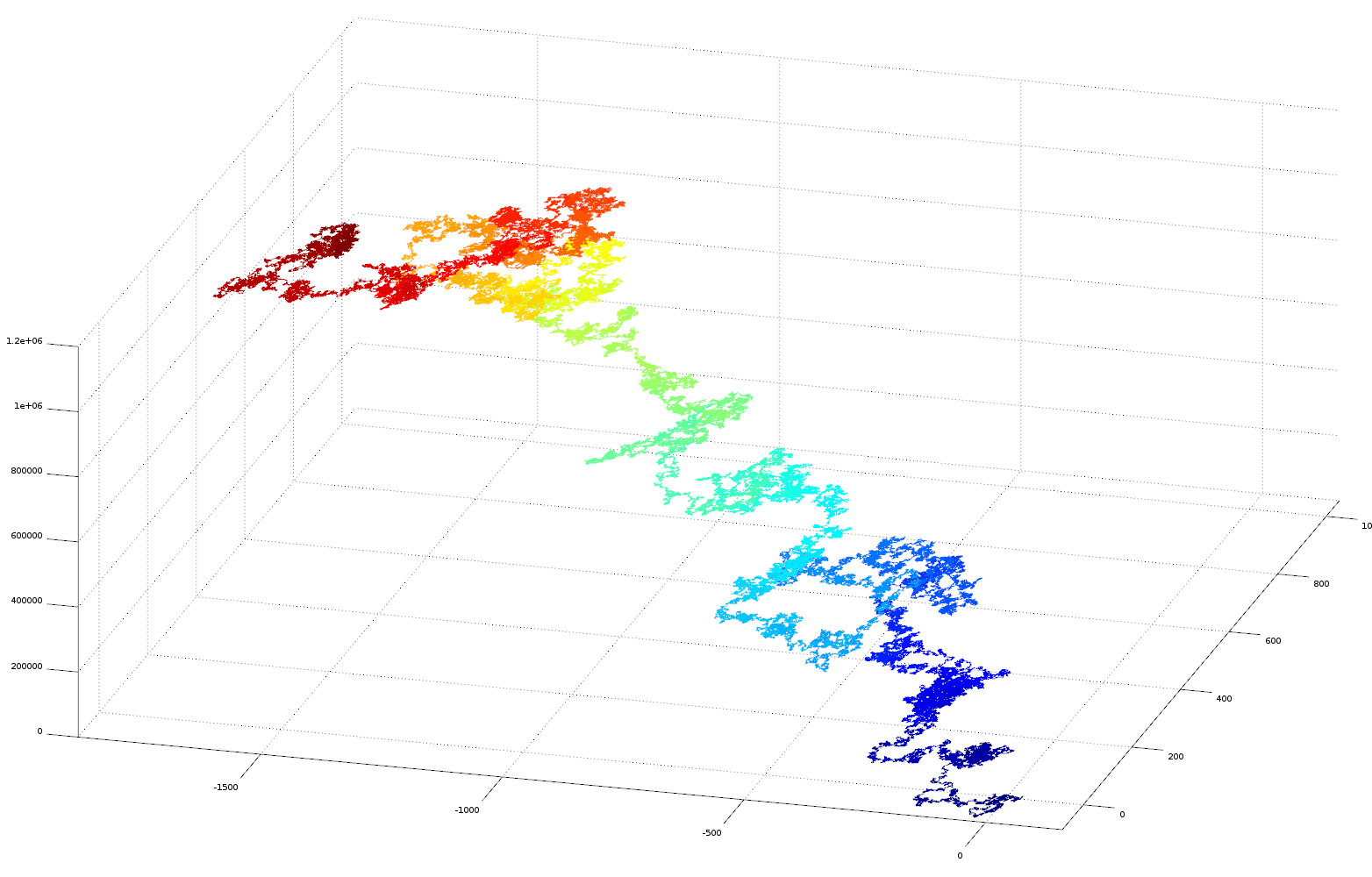
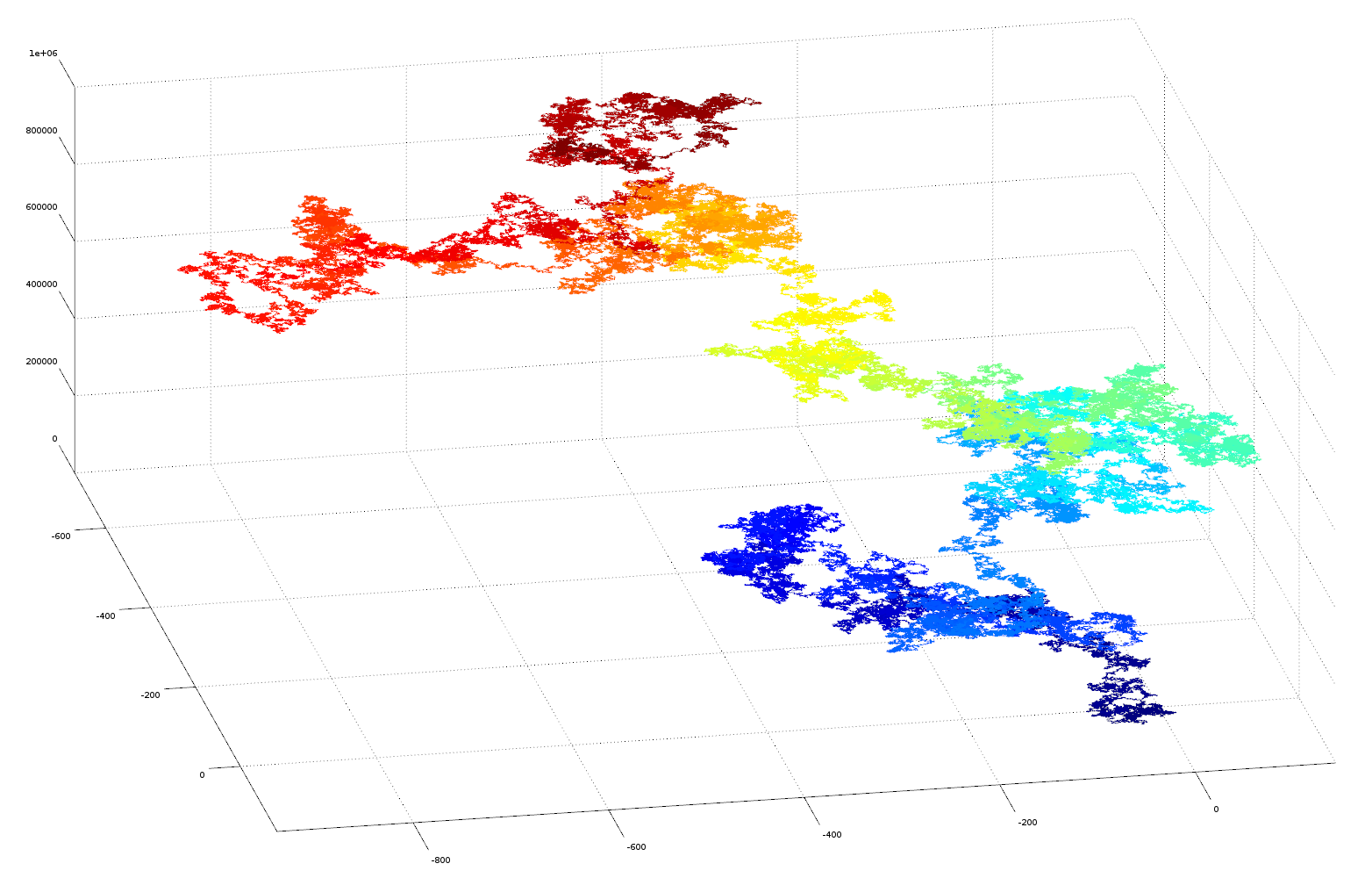
In this experiment the fractional parts of the irrational numbers, pi, e, sqrt2 and golden ratio are transformed into vectors in cartesian space for visualisation purposes. Each digit of the number sequence (from left to right) is transformed into a spatial vector with unit length. The orientation is calculated from the number as: angle = (digit/10)*2*pi. Sine and cosine functions are used to derive a position in the cartesian plane relative to the position of the previous digit (see code below for more details). As the irrational number is described to greater precision its decimal place increases, this occurs on the number string from left to right. As we are traversing the number sequence this corresponds to increasing time steps of the number analysis. On the plots the sequence position of the digit (its decimal place) is colour coded using a heat mapping (blue->red on increasing significant digits). The 3D plots also gives the sequence position of the digit on the Z axis, this helps to separate overlapping sequences in cartesian space.

Visualisation/Results

These plots are the results of the analysis, please click them for more detail
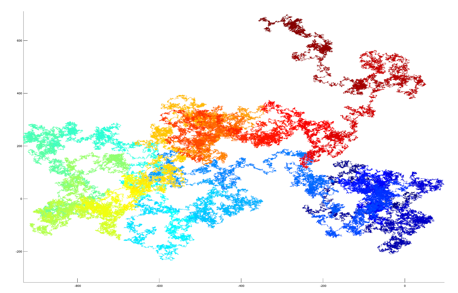
2D plot of pi as vector 3D plot of pi as vector
Fractional part of pi as a vector (colour blue->red (and Z axis) represents increasing number of decimal places) click to see enlarged image.
2D plot of pi as vector 3D plot of pi as vector
Fractional part of goldenratio as a vector (colour blue->red (and Z axis) represents increasing number of decimal places) click to see enlarged image.
2D plot of pi as vector 3D plot of pi as vector
Fractional part of sqrt2 as a vector (colour blue->red (and Z axis) represents increasing number of decimal places) click to see enlarged image.
2D plot of e as vector 3D plot of e as vector
Fractional part of e (natural logarithm base) as a vector (colour blue->red (and Z axis) represents increasing number of decimal places) click to see enlarged image.

Here is a vector plot of 1 million random number generated numbers
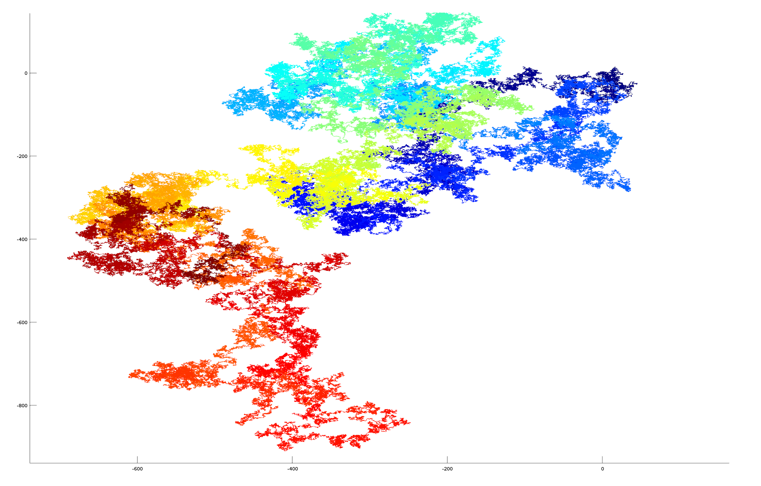
2D plot of e as vector 3D plot of e as vector
Random numbers as a vector (colour blue->red (and Z axis) represents random digits in time generated by the Octave random number generator) click to see enlarged image.

Data and Matlab/Octave computer code

Below is the Matlab/Octave code used for generating the plots. Data can be downloaded here: pi, e, golden ratio, sqrt2 (data is without decimal point!)

function  irrational_number_plot_as_vector(filepathname)
%   requires file name containing string of irrational number delete decimal point from string ie 3.14... -> 314... 

% read text file containing number
format = "%1c"

fileID = fopen('pi.txt','r');

p = fscanf(fileID, format);

_p=0;

% convert character string to matlab array
for i=1:length(p); _p(i)  = str2double(strcat(p(i),".0")); end

% create arrays for plotting
x_array = zeros(1,length(_p));
y_array = zeros(1,length(_p));

% polar angle
for i=2:length(_p); x_array(i) = x_array(i-1)+cos((_p(i-1)/10.0)*2.0*pi); y_array(i) = y_array(i-1)+sin((_p(i-1)/10.0)*2.0*pi); end

% surface plot with z axis and colour blue->red as increased fractional part
h = surface([x_array(:), x_array(:)], [y_array(:), y_array(:)], [[1:length(_p)]', [1:length(_p)]'], [[1:length(_p)]', [1:length(_p)]'], 'EdgeColor','flat', 'FaceColor','none');

end
Understanding mortgages/loans

How mortgages or loans companies make money from you

The reason for this article is that in the past (whilst living in the UK) I have moved location and bought another house somewhere else like many people do. The mortgage company or bank said that they must cancel the mortgage and take out a new mortgage on the new house. It surprised me how little money I received back from the bank for the old mortgage for all those months that I had paid X hundreds of pounds paying back the mortgage (excluding the additional penalties for early termination!). So this article is going to look at the mortgage payments and give a few plots to illustrate what happens with your money.

In our mortgage example we are going to borrow 140,000 pounds at an interest of 6.5% annually for a term lasting 30 years. The main calculation will be how much of the principal (amount borrowed is paid back every month). For this we will use the annuity formula, where `r` is the monthly interest rate expressed as a decimal (`r`=yearly_rate/12/100), `P` is the principal or the amount borrowed and `N` the number of months in the full term.

`c=(r*P)/((1-(1+r)^-N))`

Using this formula we can calculate our monthly payment (c=885 pounds). The other formula we need is for the debt schedule which tells us how much of the principal gets paid off every month which we will term `p`.

`p=((1+r)*P’)-c`

Where `P’` is the previous months outstanding amount (`p`) which at the beginning of the term will be equal to `P` (More information on the formulas used can be found here).

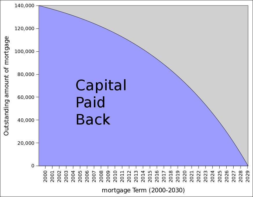
I have generated a few plots from the formulas given above to try to demonstrate what happens to your money when you pay back a mortgage or loan. For example the plot of `p` vs `N` below shows a typical repayment curve for the borrowed money

capital outstanding
How the capital amount owed decreases with time

You can see in this figure that the amount of the capital that you pay back in the beginning years is not much with most of the money being spent paying back the interest. This means that if you move early on in the term you wont get much money back from the mortgage, therefore it is better if possible to hang in there until the full term has ended.

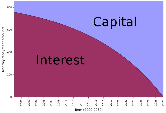
The next figure shows the proportions of the monthly mortgage payment split between capital and interest payments as the mortgage progresses. It actually takes 19 years 4 months before capital payments are greater than the interest payments in a 30 year mortgage.

monthly repayment fractions
Proportions of monthly mortgage payment that goes towards paying capital vs interest payments

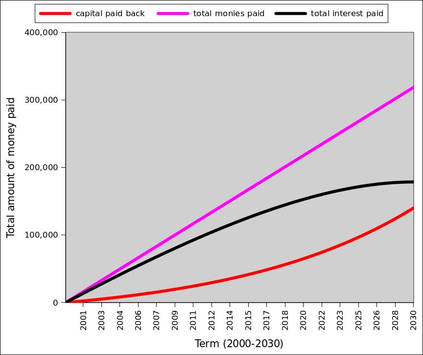
The final figure shows just how much extra money is made from lending the money and which proportion of this is interest or capital repayment. You actually pay more money towards interest than you do towards capital and the total money spent during the mortgage term is more than double the money borrowed.

total amount of money paid
Total Amount of money paid during lifetime of mortgage

Thank you Wikkipedia, Gnumeric and MathJax

Tutorial using Matlab to show how to perform transforms in 3D from one coordinate system to another

For real world vision or Robotic operations it is sometimes necessary to transform between coordinates in different coordinate systems. In this tutorial we will transform a 3D spiral from one coordinate system to another. The coordinate systems are specified in terms of their position in Cartesian space and converted to a vectorial representation.

First let us create and display the spiral


t = 0:pi/50:10*pi;
st = sin(t);
ct = cos(t);

The spiral is in 3D but we need a 4D matrix to perform the matrix transformations, so we also add a row of ones to it


spiral = [st; ct; t; ones(501,1)']

Ok, lets plot the relevant data


plot3(spiral(1,:), spiral(2,:), spiral(3,:), 'b')

we use the hold on command to keep plotting to the same chart


hold on

We are going to translate this spiral from its world coordinates to another local coordinate system

the coordinates are specified by a matrix = [X1, X2, X3, Y1, Y2, Y3, Z1, Z2, Z3]


world = [1,0,0;0,1,0;0,0,1]
local = [3,6,3;3,3,6;3,3,0]

The 3,3,0 in the last row (Z axis) of the matrix creates a 45 degree plane

Lets turn our local coordinate system into a vector


local_vector = zeros(3,3)
local_vector(:,1) = local(:,2)-local(:,1)
local_vector(:,2) = local(:,3)-local(:,1)
local_vector(:,3) = cross(local_vector(:,1),local_vector(:,2))

The vectors should be normalised to unit length like our world vector is


local_vector(:,1) = local_vector(:,1)/norm(local_vector(:,1))
local_vector(:,2) = local_vector(:,2)/norm(local_vector(:,2))
local_vector(:,3) = local_vector(:,3)/norm(local_vector(:,3))

Now we have to create our transform matrix using the dot product between our world and local vectors, this sets up the skew, reflection, rotation elements


transform = zeros(4,4)
transform(1,1) = dot(world(1,:), local_vector(1,:))
transform(1,2) = dot(world(1,:), local_vector(2,:))
transform(1,3) = dot(world(1,:), local_vector(3,:))
transform(2,1) = dot(world(2,:), local_vector(1,:))
transform(2,2) = dot(world(2,:), local_vector(2,:))
transform(2,3) = dot(world(2,:), local_vector(3,:))
transform(3,1) = dot(world(3,:), local_vector(1,:))
transform(3,2) = dot(world(3,:), local_vector(2,:))
transform(3,3) = dot(world(3,:), local_vector(3,:))

we also add the translated origin of our coordinate system to the last column of the matrix, this performs the X,Y,Z translation


transform(1,4) = local(1,1)
transform(2,4) = local(2,1)
transform(3,4) = local(3,1)
transform(4,4) = 1

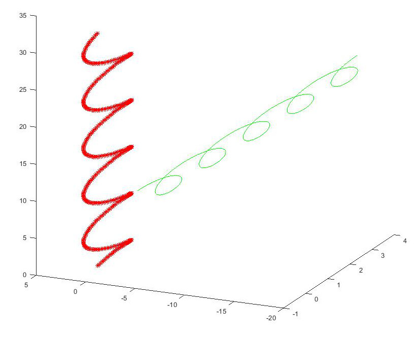
So using our transform we can rotate the spiral by 45 degrees and translate it by 3 in X and 3 in Y


tspiral = transform*spiral;

let’s plot it in green next to the original spiral


plot3(tspiral(1,:), tspiral(2,:), tspiral(3,:), 'g')

(you might want to rotate the plot axis now to see the two spirals in 3D)

now to get it back again we use the inverse of our transformation matrix


tunspiralInv = inv(transform)*tspiral;

and plot it using markers so we can see the orginal spiral beneath

plot3(tunspiralInv(1,:), tunspiralInv(2,:), tunspiralInv(3,:), ‘r*’)

The plot should look like this

plot of spiral being translated between coordinate systems

For the mathematical details behind the transform, these MIT lecture notes provide an excellent explanation.

If you find the article useful, please feel free to post a link to it